Consider for a moment you have just taken down a group of bandits. It wasn't your fault. Those pesky bandits wouldn't let you cross their bridge without a toll and you just spent all your Septim on a powerful great sword. Now comes the hard part: looting the bodies of the bandits for profit. The problem is you are near emcumbrance and unfortunately you don't have a Fortify Carry Weight potion. Maybe you should have bought a math book instead..

What's Being Asked?
Okay, so you've fully looted the bandits and spread out everything of worth on the ground:

| Item Name | Weight (units) | Value (Septim) | |
|---|---|---|---|
| A | Long Bow | 5 | 30 |
| B | Dwarven Sword | 12 | 135 |
| C | Nord Hero Greatsword | 16 | 250 |
| D | Dwarven Greatsword | 19 | 270 |
| E | Dwarven Warhammer | 27 | 325 |
You'd love to carry everything, but you only have room to carry another 40 units of weight. By the Nine!!
Let's Get Greedy
You immediately grab the Dwarves Warhammer cause you know it will fetch the highest price at 325 Septim. That leaves you with 13 units of weight so you grab the Dwarven Sword. You now are nearly encumbered and hold 325 + 135 = 460 for profit. But then you suddenly notice the two greatswords would fetch a good value as well. You have taken a greedy approach and failed to find an optimal solution.
Greedy algorithms is an approach to solving a problem by taking the optimal choice at each stage, while attempting to find an overall optimal value. Our great hero tried this approach, but it's possible to spot the correct optimal solution. Can you spot it?
Answer: Take the two greatswords and the Log Bow, which will give you a weight of 40 and value of 550. Proving that there are times when actually want to pick up a boring old Long Bow.
Greedy algorithms are useful (see Activity Selection Problem), however we just proved that it doesn't work for our immediate problem. So where do we go from here?
Counting Combinations
The Knapsack Problem is considered a combinatorial optimization problem, therefore the immediate thought would be to start counting all the combinations possible. Before we start doing this, we should consider how much work we are actually going to have to do (computer cycles) given our input. Let's consider our 5 input items. We can either take or not take an item, therefore we should consider 2n, or 25 = 32 combinations. Our hero may spend the afternoon finding the right combination, however imagine looting 10 items. That's a total of 1,024 combinations!! Let's hope our hero packed some camping supplies.
Warning: Be sure not problem to confuse this problem with as a permutation problem. Permutations are combinations while considering order. In other worsd, Red-Green-Blue does not equal Blue-Green-Red. When counting permutations use
n!, so5! = 120permutations.
Top-Down Approach
Let's consider for a moment you haven't taken any loot yet and you have a total of 40 units of weight available. Starting with the Long Bow (Item A), you naturally have two options:
- Take the Long Bow adding 5W / 30V to your knapsack.
- Do not take the Long Bow, and continue on to the second item.
Provided your character's intelligence is high enough so that his/her head doesn't explode, realize that you have essentially created two path from which to follow. This pattern continues until:
- You inventory is full capacity (encumbered).
- You have exhausted all items to add.
Let's examine a visual representation of what our decision tree would look like. When we take an item we move left down the tree and right when we don't take an item. Notice that some boxes have matching colors. These colors represents duplicate combinations, and also shows why taking a top-down approach is not so efficient (combined with the fact that you might overflow your stack if the input size is very large).
{% include utils/image.html src="/assets/collections/problems/I_O Knapsack Problem - Top-Down.png" %}
Visual representation of I/O Knapsack recursive tree.
Here is the code for this approach:
def knapsack(w: list, v: list, wt: int, idx: int = 0) -> int:
  if wt == 0 or idx == len(w):
    """
    Base Case 1: Weight capacity reached
    Base Case 2: No more items to add
    """
    return 0

  if w[idx] > wt:
    """
    Weight of item in question too heavy to take..
    """
    return knapsack(w, v, wt, idx + 1)

  """
  Finally, compare the decision of taking or not taking..
  """
  take  = v[idx] + knapsack(w, v, wt - w[idx], idx + 1)
  leave = knapsack(w, v, wt, idx + 1)

  return max(take, leave)

print(
  knapsack(
    [5, 12, 16, 19, 27],       # Item weights
    [30, 135, 250, 270, 325],  # Item values
    40                         # Available capacity
  )
)
# => 550
Note: our
knapsackfunction only returns the optimal value, and not which items make up this value.
Bottom-Up Approach
Unfortunately our hero doesn't have the computing power (intelligence) available to solve the problem using the top-down approach. Let's examine a more elegant approach that doesn't involve recursion.
Remember the base case from above was one of either two scenarios:
- You inventory is full capacity (encumbered).
- You have exhausted all items to add.
Therefore, we'll start with a similar scenario of having 0 extra inventory space and 0 items to pick up. Yes, this sounds strange at first. Why consider such a scenario when we know the optimal solution is 0 (i.e. no items to carry and no inventory space)? Let's make things a bit more interesting by slowly increasing one (of two possible) inputs (e.g. increasing weight capacity by 1 unit). By doing this we introduce subproblems that are easier to solve than the whole.
For this example, we'll be using the following information (for brevity sake):

Let's start by increasing the capacity by 1 until we get to the max capacity of 8, still with 0 items:
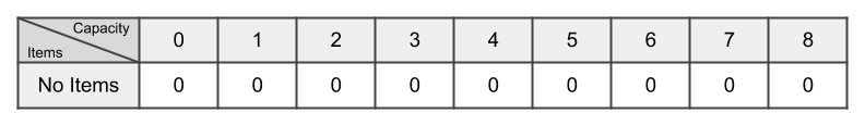
Pretty simple. Since there are no items to add, obviously the value won't increase. Now we add Item A to the chart:
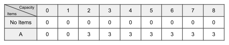
Starting at 2kg we finally have available space to take Item A (at a weight of 2kg). This continues for the rest of the row. Now things start to get interesting when we add Item B to the mix:
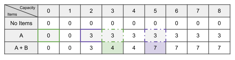
When we arrive at 3kg and 7kg we are tasked with finding an optimal solution of either taking Item B or not taking Item B. We can visually represent both decision pictured above by the following diagram:

Starting with 3kg, the decision to take Item B leaves no room in the sack for Item A and thefore the total value comes to \$4. Not taking Item B will leave 3kg in the sack leaving us with the previous optimal solution of \$3 (directly up one row). Moving on to 5kg, we are faced with the same decision. We obviously want to take both Item A & B as they add up to 5kg.
Finally, we now add Item C to the diagram:
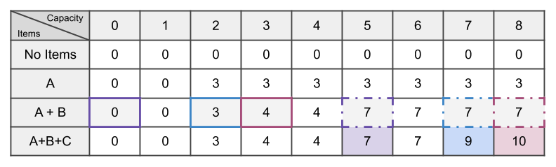
Again, we can visiually show the pertinent decisions in the table above in the diagram below:
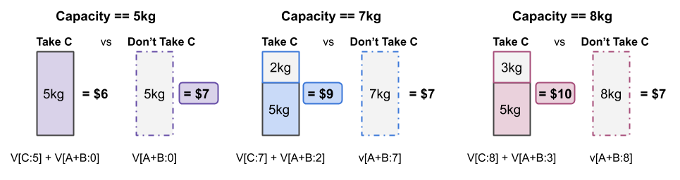
We're done! The optimal value for an 8kg sack with Items A, B, & C is \$10. It's finally time to write some code:
def knapsack(w: list, v: list, wt: int, n: int) -> int:
  # pre-generate 2D array upfront..
  arr   = [[0 for i in range(wt + 1)] for j in range(n + 1)]
  items = []

  # Genrate optimized 2D array.
  def optimized2DArray():
    for i in range(1, n + 1):                # Adding items  (i)
      for j in range(wt + 1):                # Adding weight (j)
        value    = v[i - 1]                  # Current item's value
        weight   = w[i - 1]                  # Current item's weight
        previous = arr[i - 1][j]             # Previous optimal value

        if weight > j:                       # Item too heavy!
          arr[i][j] = previous               # Copy cell immediatly above.
        else:                                # ...else...
                                                       # Compare take vs not take
                                                       #   and take max value.
          arr[i][j] = max(value + arr[i - 1][j - weight], previous)

  # Determine items selected from optimized 2D array.
  def findItems():
    j = wt

    for i in range(n, 0, -1):
      if arr[i][j] > arr[i - 1][j]:
        items.append(i)
        j -= w[i - 1]

    return items

  optimized2DArray()
  findItems()

  return items, arr[n][wt]

print(
  knapsack([2, 3, 5], [3, 4, 6], 8, 3)
)
# => ([3, 2], 10)
Voila! We have the optimal value and also which items have been added to our sack. Try it yourself with our original example and see if you can get the correct answer. After all, our brave and nobel hero would love to get back to town to sell some loot.

Conclusion
Dynamic Programming is a powerful approach when solving optimization problems. The trick is to start small (e.g. one or more base cases) and adjust your input to find the global optimized solution. The optimal solution at each point in time can be determined using the functional equation. The functional equation in our example above was:
arr[i][j] = max(value + arr[i - 1][j - weight], previous)
In this line of code we considered two options: taking an item and not taking an item using previous knowledge we uncovered.
Reference
- Algorithm Lecture 18: Dynamic Programming, 0-1 Knapsack Problem - Guided walkthrough of the Factorial and I/O Knapsack problem.
- Dynamic Programming - Examples: Computer Algorithms - Some problems to try using the Dynamic Programming approach.